TLDR

This project was developed by my team as part of our Bangkit Capstone Project. It is an Android application that uses an image classification model to identify different categories of waste. Based on the detected waste category, the application recommends suitable craft tutorials to help users creatively reuse or recycle the waste materials.

I contributed as a Machine Learning cohort member by developing an image classification model capable of detecting different categories of waste. The model serves as the core component of the application, enabling it to recommend appropriate craft tutorials based on the detected waste category.

Model Training Workflow

The overall workflow consists of the following stages: data gathering, data labeling and cleaning, model training, training the, and testing the trained model using new images.

Data Gathering

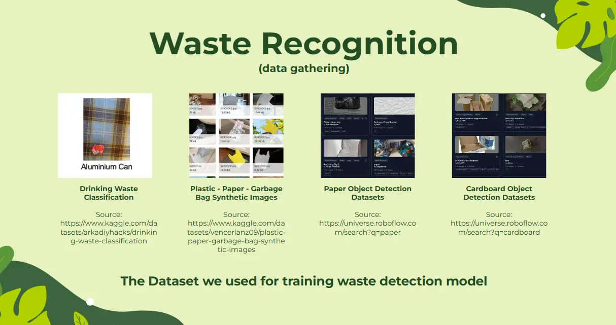
The data gathering stage involves collecting images of various types of waste, including plastic, paper, glass, and organic waste. The dataset was assembled from multiple sources, primarily Kaggle and Roboflow, to ensure sufficient diversity and coverage for training the image classification model.

Data Labeling and Cleaning

For the data labeling and cleaning stage, I used Roboflow, a platform that simplifies dataset management, annotation, and preprocessing. It provides an intuitive interface for organizing large image datasets, making it much more efficient than manually managing files.

When labeling a large number of images, it is not always necessary to annotate every image manually. Roboflow supports assisted annotation workflows, including AI-powered labeling models that can automatically generate annotations, significantly reducing the time and effort required.

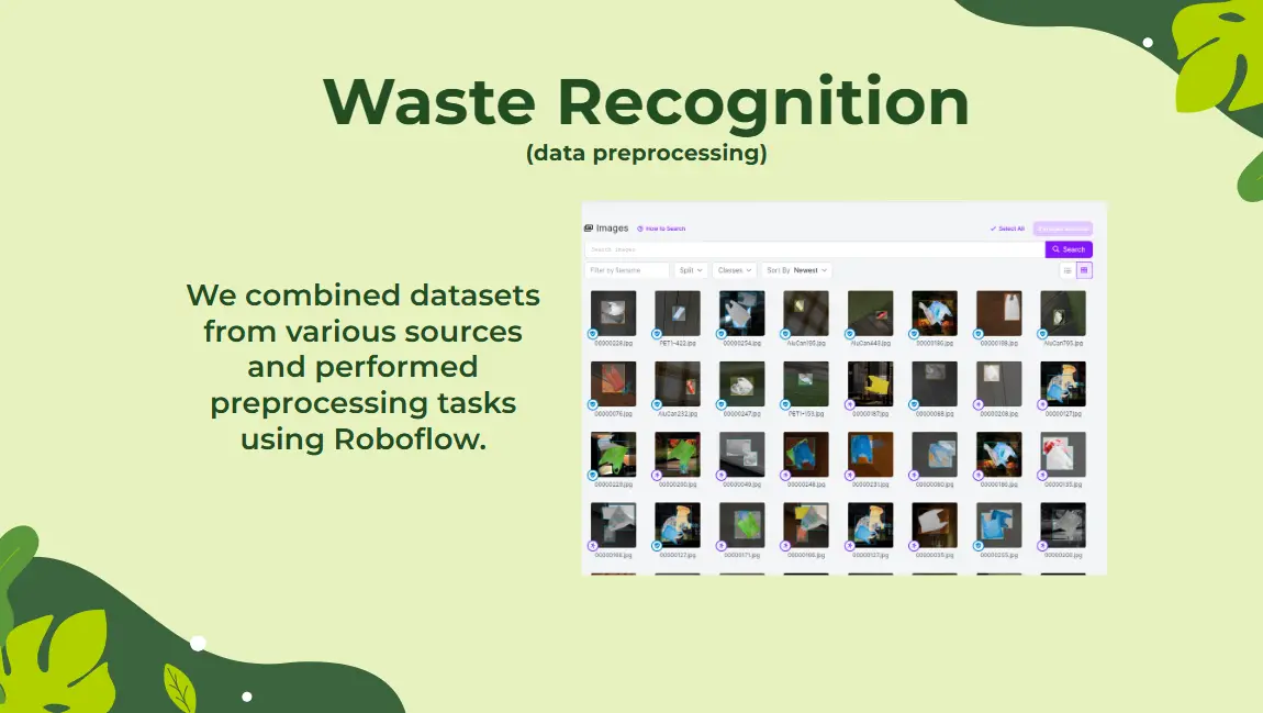
Another advantage of Roboflow is its dataset versioning and export capabilities. It provides a Python package and API that allow datasets to be downloaded directly into the training environment. After the dataset has been cleaned and finalized, it can be retrieved programmatically with just a few lines of code. This feature will be discussed in more detail in the Model Training stage.

Model Building

Rather than training a model from scratch, I adopted a transfer learning approach by using MobileNetV2 pretrained on the ImageNet dataset as the feature extractor. MobileNetV2 was chosen because it is a lightweight convolutional neural network designed for resource-constrained devices, making it well suited for deployment on Android smartphones while still delivering strong image classification performance.

To adapt the model to the waste classification task, I froze the pretrained MobileNetV2 layers so that the learned feature representations remained unchanged during training. On top of the feature extractor, I added several custom convolutional layers, followed by a Global Average Pooling layer and fully connected layers to learn features specific to the waste categories in the dataset.

The model was trained using the Adam optimizer with a learning rate of 1 × 10⁻⁵. Since the dataset contained an imbalanced distribution of classes, I computed class weights using scikit-learn and applied them during training. This helped reduce the bias toward majority classes and encouraged the model to learn minority classes more effectively.

Training was performed for 30 epochs, while model performance was monitored using the AUC (Area Under the ROC Curve) and F1-score metrics. These metrics provide a more informative evaluation than accuracy alone, especially when working with imbalanced datasets.

Here the preview how I build that model

Preparing the packages

I start by importing the required libraries.

!pip install tensorflow-addons
import os
import tensorflow as tf
import tensorflow_addons as tfa
import numpy as np
import pandas as pd
import random
import cv2
import sklearn
import matplotlib.pyplot as plt
import matplotlib.style as style
from google.colab import files

Preparing the Dataset

After the dataset had been labeled and cleaned in Roboflow, the next step was to prepare it for model training. This stage involved downloading the dataset, loading the annotations into memory, performing basic preprocessing, and creating data generators that would feed images to the neural network during training.

Download the Cleaned Dataset

Roboflow provides an API that allows datasets to be downloaded directly into the training environment. This eliminates the need to manually export and upload datasets whenever changes are made. The following commands remove any previous dataset, download the latest version from Roboflow, and extract it into a dedicated dataset directory.

!rm -r dataset
!rm data
!wget https://app.roboflow.com/ds/gzGSPSpsan?key=CrzyeSBgrQ
!mv gzGSPSpsan?key=CrzyeSBgrQ data
!mkdir dataset
!unzip data -d dataset

Load the Dataset

After downloading the dataset, the training and validation annotation files (_classes.csv) are loaded into Pandas DataFrames. These CSV files contain the image filenames together with their corresponding labels. The paths to the training and validation image directories are also stored for use when creating the data generators.

dataset_dir = os.path.join(os.getcwd(), 'dataset')
train_label_df = pd.read_csv(os.path.join(dataset_dir, 'train', '_classes.csv'))
validation_label_df = pd.read_csv(os.path.join(dataset_dir, 'valid', '_classes.csv'))
train_images_dir = os.path.join(dataset_dir, 'train')
validation_images_dir = os.path.join(dataset_dir, 'valid')

Data Preprocessing

Before creating the data generators, the column names are cleaned by removing unnecessary whitespace. This ensures that the label names are consistent and can be referenced correctly throughout the training process.

train_label_df.columns = train_label_df.columns.str.strip()
validation_label_df.columns = validation_label_df.columns.str.strip()

Next, the waste categories are defined, and TensorFlow's ImageDataGenerator is used to normalize the pixel values of each image from 0–255 to 0–1 using the rescale parameter. Normalization helps the neural network train more efficiently and improves numerical stability during optimization.

The dataset is loaded using flow_from_dataframe, which reads images directly from disk in batches instead of loading the entire dataset into memory. This approach is more memory-efficient and scales well for larger datasets.

Since this project performs multi-label image classification, the generators use class_mode='raw'. Unlike single-label classification, where each image belongs to exactly one class, a multi-label dataset allows an image to contain multiple waste categories simultaneously. Each label is represented as a binary vector, enabling the model to learn the presence or absence of every waste category independently. This configuration is compatible with the model's sigmoid output layer and the binary cross-entropy loss function used during training.

columns = [
    "aluminiumfoil",
    "bottle",
    "bottlecap",
    "can",
    "carton",
    "cup",
    "paper",
    "plastic",
    "straw"
]
 
train_datagen = tf.keras.preprocessing.image.ImageDataGenerator(
    rescale=1./255.
)
 
validation_datagen = tf.keras.preprocessing.image.ImageDataGenerator(
    rescale=1./255.
)
 
if os.path.exists(train_images_dir):
    train_generator = train_datagen.flow_from_dataframe(
        dataframe=train_label_df,
        directory=train_images_dir,
        x_col='filename',
        y_col=columns,
        batch_size=32,
        seed=42,
        class_mode='raw',
        shuffle=True,
    )
 
if os.path.exists(validation_images_dir):
    validation_generator = validation_datagen.flow_from_dataframe(
        dataframe=validation_label_df,
        directory=validation_images_dir,
        x_col='filename',
        y_col=columns,
        batch_size=32,
        class_mode='raw',
        seed=42,
        shuffle=False,
    )

Model Training

To build the waste classification model, I adopted a transfer learning approach using MobileNetV2 pretrained on the ImageNet dataset as the feature extractor. MobileNetV2 was selected because it is a lightweight convolutional neural network designed for mobile and embedded devices, making it well suited for Android applications while still providing strong classification performance.

Instead of training the entire network from scratch, the pretrained feature extractor is frozen so that its learned visual representations remain unchanged. This allows the model to focus on learning features that are specific to the waste classification task while reducing training time and the risk of overfitting.

feature_extractor = tf.keras.applications.MobileNetV2(
    include_top=False,
    weights='imagenet',
    input_tensor=tf.keras.Input(shape=(640, 480, 3))
)
 
feature_extractor.trainable = False

After obtaining the feature extractor, several custom convolutional layers are added to further learn task-specific features from the waste dataset. The extracted features are then compressed using a Global Average Pooling layer before being passed to a fully connected layer.

The output layer consists of 9 neurons with a sigmoid activation function because this project performs multi-label image classification. Unlike a softmax activation, sigmoid predicts an independent probability for each class, allowing the model to identify multiple waste categories within a single image.

inputs = tf.keras.layers.Input(shape=(640, 480, 3))
x = feature_extractor(inputs)
x = tf.keras.layers.Conv2D(filters=64, kernel_size=(3, 3), activation='relu', padding='same')(x)
x = tf.keras.layers.MaxPooling2D((2, 2))(x)
x = tf.keras.layers.Conv2D(128, (3, 3), activation='relu', padding='same')(x)
# x = tf.keras.layers.MaxPooling2D((2, 2))(x)
x = tf.keras.layers.Conv2D(256, (3, 3), activation='relu', padding='same')(x)
# x = tf.keras.layers.MaxPooling2D((2, 2))(x)
x = tf.keras.layers.Conv2D(512, (3, 3), activation='relu', padding='same')(x)
x = tf.keras.layers.MaxPooling2D((2, 2))(x)
 
x = tf.keras.layers.GlobalAveragePooling2D()(x)
x = tf.keras.layers.Dense(1024, activation='relu')(x)
# x = tf.keras.layers.Dropout(0.5)(x)
outputs = tf.keras.layers.Dense(9, activation='sigmoid')(x)
 
model = tf.keras.Model(inputs=inputs, outputs=outputs)

The model is compiled using the Adam optimizer with a learning rate of 1 × 10⁻⁵. Since this is a multi-label classification problem, binary cross-entropy is used as the loss function. Model performance is evaluated using AUC (Area Under the ROC Curve) and F1-score, both of which provide a more informative assessment than accuracy, particularly when working with imbalanced datasets.

model.compile(
    tf.keras.optimizers.Adam(learning_rate=0.00001),
    loss='binary_crossentropy',
    metrics=[
        tf.keras.metrics.AUC(name='auc'),
        tfa.metrics.F1Score(
            num_classes=1,
            average='micro',
            name='f1_score'
        )
    ]
)

Before training, class weights are computed to address the imbalance in the dataset. Minority classes receive larger weights during optimization, encouraging the model to learn them more effectively and reducing bias toward the majority classes.

train_labels = []
 
for _ in range(len(train_generator)):
    _, batch_labels = next(train_generator)
    train_labels.extend(batch_labels)
 
train_labels = np.array(train_labels)
train_labels = np.argmax(train_labels, axis=1)
 
class_weights = sklearn.utils.class_weight.compute_class_weight(
    class_weight='balanced',
    classes=np.unique(train_labels),
    y=train_labels
)
 
class_weights_dict = dict(enumerate(class_weights))

Finally, the model is trained for 30 epochs using the training dataset while evaluating its performance on the validation dataset after each epoch. The previously computed class weights are applied throughout training to help improve the model's ability to recognize underrepresented waste categories.

_history = model.fit(
    train_generator,
    epochs=30,
    validation_data=validation_generator,
    class_weight=class_weights_dict
)

Testing the Trained Model with New Images

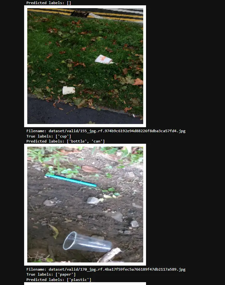
After the training process was completed, the model was evaluated using images from the validation dataset to observe how well it generalized to unseen data. Rather than evaluating only numerical metrics, I also performed a qualitative inspection by comparing the model's predictions with the ground truth labels.

First, the model generates probability scores for each waste category. Since this is a multi-label classification task, each output neuron produces an independent probability indicating the likelihood that a particular waste category is present in the image.

predictions_prob = model.predict(validation_generator)
 
print("Predicted probabilities for the first sample:")
print(predictions_prob[0])

To convert the predicted probabilities into class labels, a threshold of 0.5 is applied. Categories with probabilities greater than the threshold are considered present in the image, while the remaining categories are ignored.

threshold = 0.5
 
predictions_binary = (predictions_prob > threshold).astype(int)
validation_filenames = validation_generator.filenames

Finally, twenty random images are selected from the validation dataset. For each image, the corresponding ground truth labels and the model's predicted labels are displayed alongside the image itself. This visual comparison provides an intuitive way to assess the model's performance and identify cases where the predictions are correct or where further improvements may be needed.

# Random 20 images
random_indices = random.sample(range(len(validation_filenames)), 20)
 
print(random_indices)
 
for index in random_indices:
    image_path = os.path.join('dataset', 'valid', validation_filenames[index])
 
    image = tf.keras.preprocessing.image.load_img(
        image_path,
        target_size=(224, 224)
    )
 
    # Get the corresponding labels and predictions
    labels = validation_generator.labels[index]
    predicted_labels = predictions_binary[index]
 
    # Display the image
    plt.imshow(image)
    plt.axis('off')
 
    print("Filename:", image_path)
    print(
        "True labels:",
        [columns[k] for k, label in enumerate(labels) if label == 1]
    )
    print(
        "Predicted labels:",
        [columns[k] for k, label in enumerate(predicted_labels) if label == 1]
    )
 
    plt.show()

The results showed that the trained model was able to correctly identify the waste categories for most validation images. Comparing the predicted labels with the ground truth labels also helped verify that the model had successfully learned meaningful visual features and generalized well beyond the training dataset.

The Final Result

After the model was successfully trained and evaluated, it was handed over to the Cloud Computing team for deployment. Their responsibility was to prepare the backend service that exposed the model through an API, allowing the Mobile Development team to integrate the image classification feature into the Android application.

This collaboration enabled the machine learning model to be used in the final application. Users can capture or upload an image, and the application classifies the waste before recommending a suitable craft tutorial based on the detected category.

The following screenshot shows the final implementation of the waste classification feature in the Android application: